
In the latest edition of “The Slice,” a blog series from Arize that explains the essence of ML concepts in a digestible question-and-answer format, we dive into how to calculate AUC – and where it’s most useful. Want to see AUC in the Arize platform? Sign up for a free account.
Introduction: What Is the AUC ROC Curve In Machine Learning?
AUC, short for area under the ROC (receiver operating characteristic) curve, is a relatively straightforward metric that is useful across a range of use-cases. In this blog, we present an intuitive way of understanding how AUC is calculated.
How Do You Calculate AUC?
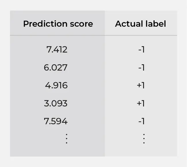
To calculate AUC, we need a dataset with two columns: prediction score and actual label (i.e. Table 1). Since the actual label is binary in this case, we use +1 and -1 to denote the positive and negative classes, respectively. The important thing to note here is that the actual labels are determined by the real world, whereas the prediction scores are just some numbers that we come up with, usually with a model.
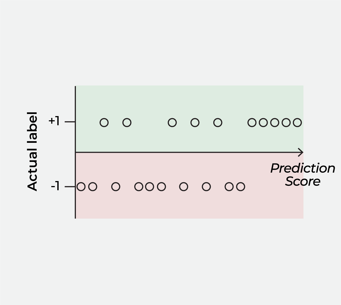
To see the AUC calculation clearly, we first visualize Table 1 as Figure 1, where each data point is plotted with its prediction score on the x-axis and the actual label on the y-axis. We do this to divide the data points into two groups identified by their actual labels, because the next step is to generate prediction labels and calculate the two quantities shown in Table 2, whose denominators are precisely the counts of data points in these two groups.
| Description | Denominator | Statistical Jargon |
| % of positive actual labels that agree with the prediction labels | Number of data points with positive actual labels | True positive rate |
| % of negative actual labels disagree with the prediction labels | Number of data points with negative actual labels | False positive rate |
| Table 2. Quantities to calculate. Remember the denominators. | ||
To generate prediction labels, we pick an arbitrary cutoff for the prediction score.
- Data points with prediction scores above the cutoff are given positive prediction labels.
- Data points with prediction scores below the cutoff are given negative prediction labels.
A ROC curve is an enumeration of all such thresholds. Each point on the ROC curve corresponds to one of two quantities in Table 2 that we can calculate based on each cutoff. For a data set with 20 data points, the animation below demonstrates how the ROC curve is constructed. AUC is calculated as the area below the ROC curve.
| When the cutoff moves past a data point with an actual label that is… | The ROC curve moves… |
| Positive | Upward |
| Negative | Rightward |
| Table 3. How each data point’s actual label influences the movement of the ROC curve | |
The key takeaway here is that AUC measures the degree of separation between these two groups of data points – identified by their actual labels – when their prediction scores are plotted on the x-axis (note: different models output different prediction scores, so the distribution would look different for different models). Table 3 summarizes how the movement on the ROC curve corresponds to each data point’s actual label, and Figure 3 and 4 show how the AUC can be 1 and 0.5 respectively.
If the two groups are perfectly separated by their prediction scores, then AUC = 1 and the model score is doing a perfect job distinguishing positive actuals from negative actuals.

If the two groups are perfectly commingled, then AUC = 0.5 and the model scores are not doing a good job distinguishing positive actuals from negative actuals.
For simplicity, we present the AUC as the area under a staircase-like curve. In practice, an additional step of smoothing is often applied before the area under it is calculated.
Where AUC Is Most Useful (Example)?
AUC is useful when models output scores, providing a high-level single-number heuristic of how well a model’s prediction scores can differentiate data points with true positive labels and true negative labels. It’s often used in data science competitions because it offers an uncomplicated way to summarize a model’s overall performance – in general, a model with a substantially lower AUC value is a worse model.
One area where AUC can be particularly useful is when accuracy falls short. For example, if a model always predicts no cancer when trying to diagnose a rare type of cancer, the model would have high accuracy because it’s almost always correct (i.e. almost no one actually has the cancer). On the other hand, the model would have an AUC value of 0.5 – meaning that it’s completely useless (the 0.5 value derives from the fact that such a model would give the same prediction score for all data points – see Figure 4 for how the 0.5 value comes about).
Where Does AUC Typically Fail (Example)?
AUC is an average of true positive rates over all possible values of the false positive rate. There are times where having a high false positive rate is not desirable from a business perspective. An example of this is in fraud detection, where having a high false positive rate would mean spending a lot of money investigating claims that ultimately turn out to be non-fraudulent. It would be irrelevant to evaluate a fraud model’s performance at high false positive rates. In general, different regions of the ROC curve may be more or less relevant in different problem contexts, and two models with similar AUC scores may be significantly different in their usefulness for a specific problem.
AUC is less useful when the prediction scores are probabilities since we are interested in the accuracy of the predicted probabilities. There are situations where the predicted probability corresponds to the cost of doing business, such as in lending or insurance, and it is important to have the predicted probabilities be well-calibrated against the actual probabilities. Because the AUC calculation only depends on the ordering of the prediction scores, it knows nothing about probabilities. Two models offering very different predicted probabilities can have very similar AUC values.
Choosing the Right Model Metric
AUC is a frequently-used metric that is helpful in a variety of contexts. As always, it’s worth keeping in mind that every model metric has tradeoffs – additional context and knowing what business outcome you’re optimizing toward can make a big difference in understanding whether to use AUC or another metric to determine whether a model is underperforming.
This blog has been republished by AIIA. To view the original article, please click HERE.
Recent Comments