In the last decade, significant technological progress has been driven rapidly by numerous advances in applications of machine learning. Novel ML techniques have revolutionized industries by cracking historically elusive problems in computer vision, natural language processing, robotics, and many others. Today it’s not hyperbolic to say that ML has changed how we work, how we shop, and how we play.

While many models have increased in performance, delivering state-of-the-art results on popular datasets and challenges, models have also increased in complexity. In particular, the ability to introspect and understand why a model made a particular prediction has become more and more difficult.

Now that ML models power experiences that impact important parts of our lives, it has become even more important that we have the ability to explain how they make their predictions.

In this piece, we will lay out the different levels of ML explainability, and how each of these can be used across the ML Lifecycle. Lastly we will cover some common methods that are being used to obtain these levels of explainability.

Explainability in Training

To start, let’s cover how explainability can be used to help during the model training phase of the machine learning life-cycle. In particular, let’s begin by starting to tease apart the different flavors of ML explainability.

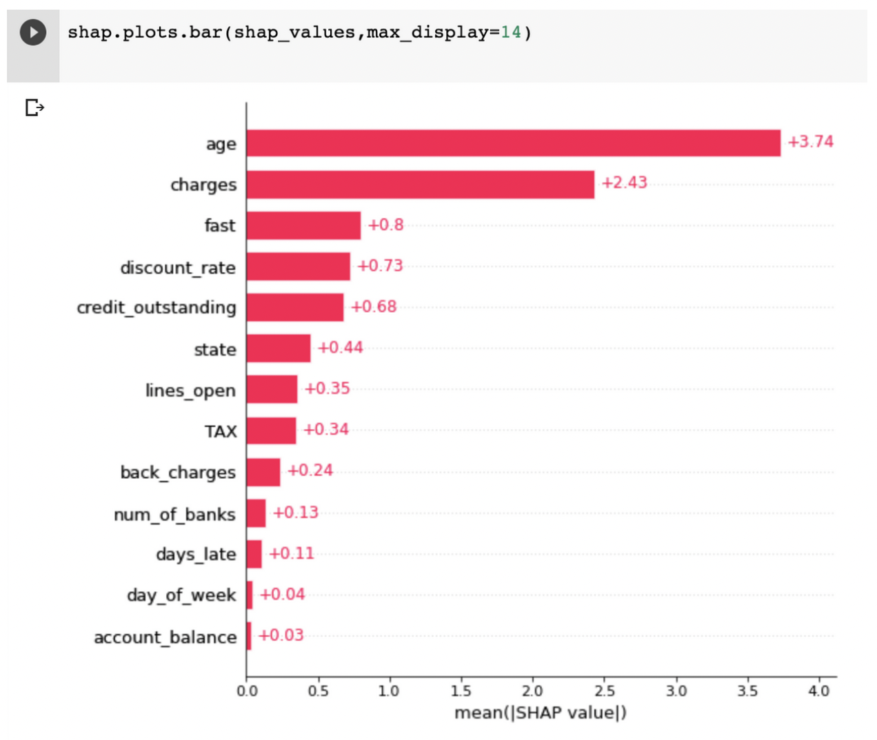
Of particular importance in training is global explainability. We consider an ML engineer to have access to global model explainability if across all predictions they are able to attribute which features contributed the most to the model’s decisions. The key term here is “all predictions,” unlike cohort or local explainability — global is an average across all predictions.

In other words, global explainability lets the model owner determine to what extent each feature contributes to how the model makes its predictions over all of the data.

In practice, one area global explainability is used is on an ad hoc basis to provide information to non-data science teams about what the model, on average, uses to make decisions. Example: marketing teams, looking at a churn model, might want to know what are the most important features to predict customer churn.

In this use case, the model provides global insights to stakeholders outside of data science, and how often it is needed and for whom can vary — it’s more of an analytical function to provide business stakeholders more insights.

There is also a model builder use case for global explainability, namely ensuring a model is doing what you expect and hasn’t changed version to version. There may be unforeseen ways your model can “learn” the function you set out to teach it, and without the ability to understand what features it’s relying on it’s hard to say which function it chose to approximate.

Let’s take a model that predicts the credit limit that a new customer should get for your bank’s new credit card. There are a number of ways that this model can accomplish its job of assigning a credit limit to this new customer, but not all are created equal. Explainability tools can help build confidence that your model is learning a function that isn’t over-indexing on particular features that may cause problems in production.

For example, let’s say a model is relying extremely heavily on age to make its prediction of what credit limit to assign. While this may be a strong predictor for ability to repay large credit bills, it may under-predict credit for some younger customers who have an ability to support a larger credit limit, or over-predict for some older customers who perhaps no longer have the income to support a high credit limit.

Explainability tools can help you find potential issues like this before shipping a model to production. Global explainability helps spot check how features in the model are contributing to the overall predictions of the model. In this case, global explainability would be able to highlight age as a primary feature that the model is relying on, and allow the model owner to understand how this might impact cohorts of their users and take action.

During training, global explainability is instrumental in gaining confidence in the features you choose to provide your model for its predictions. Often, a model builder will add a large number of features and observe a positive shift in a key model performance metric. Understanding which features or interactions between features drove this improvement can help you build a leaner, quicker, and even a more generalizable model.

Explainability in Validation

Onto the next phase of the ML lifecycle: model validation. Let’s take a look at how explainability can help model builders validate models before shipping them to production.

To this end, it’s important to define our next class of model explainability: Cohort Explainability. Sometimes you need to understand how a model is making its decisions for a particular subset of your data, also known as a cohort. Cohort explainability is the process of understanding to what degree your model’s features contribute to its predictions over a subset of your data.

Cohort explainability can be incredibly useful for a model owner to help explain why a model is not performing as well for a particular subset of its inputs. It can help discover bias in your model and help you uncover places where you might need to shore up your datasets.

Taking a step back, during validation, our primary objective is to see how our model would hold up in a serving context. To be more specific, validation is about probing how well your model has generalized from the data that it was exposed to in training.

A key component in assessing generalization performance is uncovering subsets of your data where your model may be underperforming, or relying on information that might be too specific to the data that it was trained on, also commonly known as overfitting.

Cohort explainability can serve as a helpful tool in this model validation process by helping to explain the differences in how a model is predicting between a cohort where the model is performing well versus a cohort where the model is performing poorly.

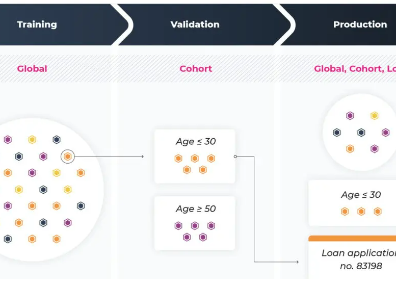
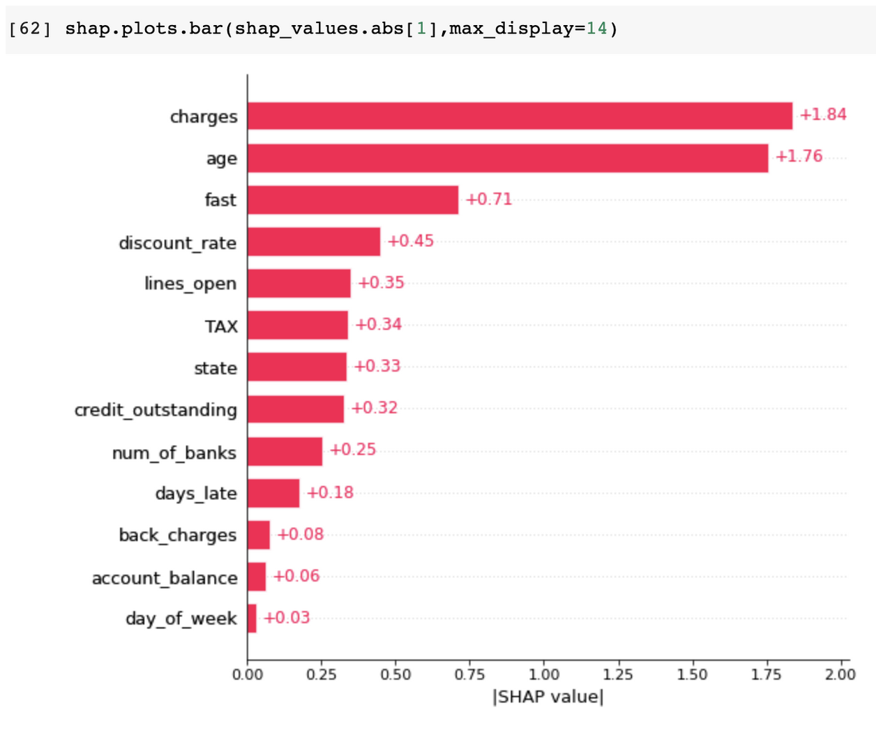
For example, let’s say that you have a model for predicting credit scores for a particular user and you want to know how the model is making its prediction for your users that are below the age of 30. It’s worth noting the most important feature for this group, “charges,” is different from the global feature importance. Cohort explainability can help investigate how your model is treating these users in comparison to some other cohort of your data, such as users above the age of 50. This can help you uncover somewhat unexpected or undesirable relationships between input features and model outcome.

Another important benefit that cohort explainability buys you is the ability to understand when to split your model into a collection of models and federate their predictions. It’s very possible that the function you are trying to learn is best handled by a federation of models, and cohort explainability can help you discover the cohorts for which a different feature set or model architecture might make more sense.

Explainability in Production

Lastly, let’s take a look at how explainability can help a model owner in the production context. Once the model has left the research lab and has been served into production, the needs of a model owner change a bit.

In production, model owners need to be able to answer all-of-the-above Cohort and Global explainability, in addition to questions about very specific examples to help with customer support, enable model auditability, or even just provide feedback to the user about what happened.

This leads us into our last class of ML explainability: Individual, also known as Local Explainability. This is somewhat self explanatory, but local explainability helps answer the question, “for this particular example, why did the model make this particular decision?”

The level of specificity is an incredibly useful tool in the toolbox for an ML engineer, but it’s important to note that having local explainability in your system does not imply that you have access to global and cohort explainability.

Local explainability is indispensable for getting to the root cause of a particular issue in production. Imagine you just saw that your model has rejected an applicant for a loan and you need to know why this decision was made. Local explainability would help you get to the bottom of which features were most impactful in making this loan rejection.

Especially in regulated industries, such as lending in our previous example, local explainability is paramount. Companies in regulated industries need to be able to justify decisions made by their model and prove that the decision was not made using features or derivatives of protected class information.

Note: In all our examples we used the absolute values of Shap for visualization; these hide the directional information of the individual features.

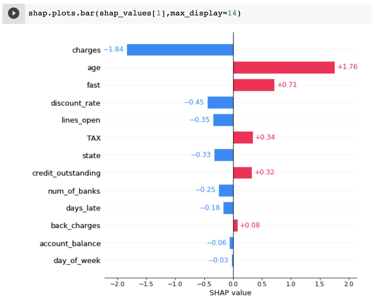
The prediction-level shap with directional information can illustrate how the feature influences an outcome — in this case, “charges” decreases the probability of default where “age” increases.

As more and more regulation impacts technology, companies are not going to be able to hide behind ML black boxes to make decisions in their products. If they would like to reap the benefits of machine learning, they are going to have to invest in solutions that provide local explainability.

When the model is served and making predictions for your users, individual inference level explainability can act as a fantastic entry point into understanding the dynamics of your model. As soon as you see a model prediction that may have gone awry, either from a bug report or monitoring thresholds that you set up, this can start an investigation into why this happened.

It may lead you to discover which features contributed most to the decision, and even cause you to dive deeper into a cohort that may also be affected by this relationship you uncovered. This can help close the ML lifecycle loop, allowing you to go from “I see a problem with an individual example” to “I have discovered a way to improve my model.”

Common Methods in ML Explainability:

Now that we have defined some broad classes of ML explainability and how they might be used in different stages of the ML Lifecycle, let’s turn our attention toward a few techniques that are powering ML explainability solutions today.

SHAP – SHapley Additive exPlanations

To start, let’s take a look at SHAP which stands for SHapley Additive exPlanations. SHAP is an explainability technique that developed from concepts in cooperative game theory. SHAP attempts to explain why a particular example differs from the global expectation from a model.

For each feature in your model, a Shapley value is computed which explains how this feature contributed to the difference between the model’s prediction for this example as compared to the “Average” or expected model prediction.

The SHAP values of all the input features will always sum up to the difference between the observed model output for this example and the baseline (expected) model output, hence the additive part of the name in SHAP.

SHAP can also provide global explainability using the Shapley values computed for each data point, and even allows you to condition over a particular cohort to gain some insight on how feature contributions differ between cohorts.

Using SHAP in the model-agnostic context is simple enough for local explainability, though global and cohort computations can be costly without particular assumptions about your model.

LIME – Local Interpretable Model-Agnostic

LIME, or Local Interpretable Model-Agnostic Explanations, is an explainability method that attempts to provide local ML explainability. At a high level, LIME attempts to understand how perturbations in a model’s inputs affect the end-prediction of the model. Since it makes no assumptions about how the model reaches the prediction, it can be used with any model architecture, hence the “model-agnostic” part of LIME.

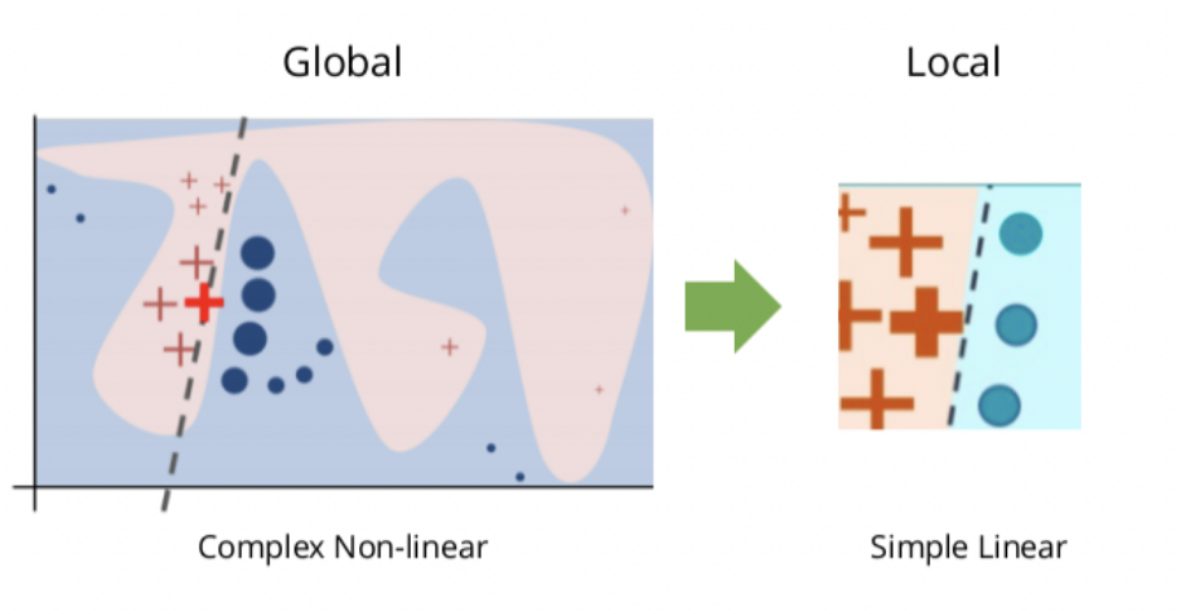
LIME attempts to understand this relationship between a particular example’s features and the model’s prediction by training a more explainable model such as a linear model with examples derived from small changes to the original input.

At the end of training, the explanation can be found from the features for which the linear model learned coefficients above particular thresholds (after accounting for some normalization). The intuition behind this is that the linear model found these features to be most important in explaining the model’s prediction, and therefore for this local example you can reason about the contributions that each feature made in explaining the prediction that your model made.

Conclusion

We are in an extremely exciting and face-paced era of machine learning, and over the last decade or so the historical roadblocks for these technologies are being upended. One of the most common critiques of modern machine learning is the absence of explainability tools to build confidence in, provide auditibability for, and enable continuous improvement of machine learned models.

Today, there is a keen interest in surmounting this next hurdle. As evidenced by some of the modern explainability techniques covered, we are well on our way.

This blog has been republished by AIIA. To view the original article, please click HERE.