
In our last post we summarized the problem of drift in machine learning deployments (“Drift in Machine Learning: Why It’s Hard and What to Do About It” in Towards Data Science). One of the takeaways from the article is: methods for dealing with drift must identify whether and how drift is consequential on model performance. A key choice that a data scientist must make in this regard is which drift metrics to employ for their particular situation. In this article, we investigate further how to select which drift metrics to use.
The Problem
Formally, suppose we have two empirical distributions (i.e. datasets): model inputs X₁ with corresponding labels Y₁; and X₂, which does not have labels yet. We can generate model outputs Ŷ₁ and Ŷ₂. We now have to decide whether *₁ differ sufficiently from *₂ to get worried about data drift, whether our model trained on X₁, Y₁ is well suited to perform well on X₂.
The data has certainly changed and, for distributions with at least a few numeric or continuous features, it is likely that there is not a single instance in common between the training and deployment inputs. We try to avoid the curse of dimensionality by looking at individual features or small sets of features at a time.
A drift metric takes in the feature values from the two data sets and gives us a measure of difference, a real number typically indicating greater difference with larger values. The questions we need to ask when deciding on the right metric include:
- Does it apply to the data type?
- Does it come with meaningful units or otherwise have a convenient interpretation?
- Does it make any assumptions about data distribution?
- Does it capture differences in small probability events / values?
- Are there ready-made implementations I can use in my projects?
In the remainder of this article we will consider these questions and several related metric criteria: what the types of features they apply to: categorical or numerical, the interpretation or underlying theory with most metrics derived from either information theory or statistics, handling of rare events, assumptions and tunable parameters. While we elaborate on each of these aspects, it is important to realize that any metric, as a summarizer of complex differences among datasets into a single number, offers only a narrow view of the type of data shifts possible.
Metrics for Feature Types
Numerical Features
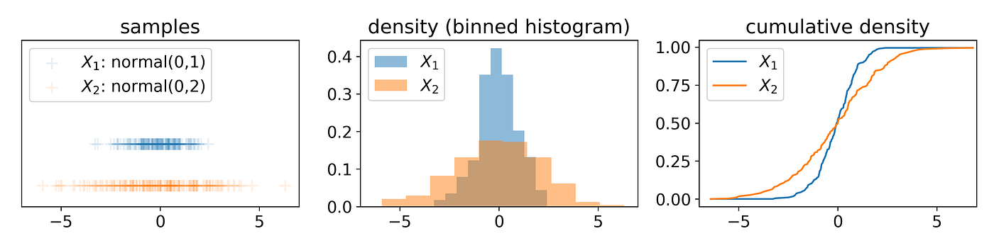
Drift metrics that measure differences among numerical features (usually) view datasets as sets of samples, binned densities, or as cumulative densities. The simplest of these merely compare common aggregate statistics such as mean across datasets:

Such metrics may be useful when the underlying data is distributed in a manner well summarized by such aggregates (i.e. if X₁ and X₂ are normally distributed, differences between means and standard deviation offer a full account of the difference between them) but data is rarely distributed nicely and these metrics may miss important differences.
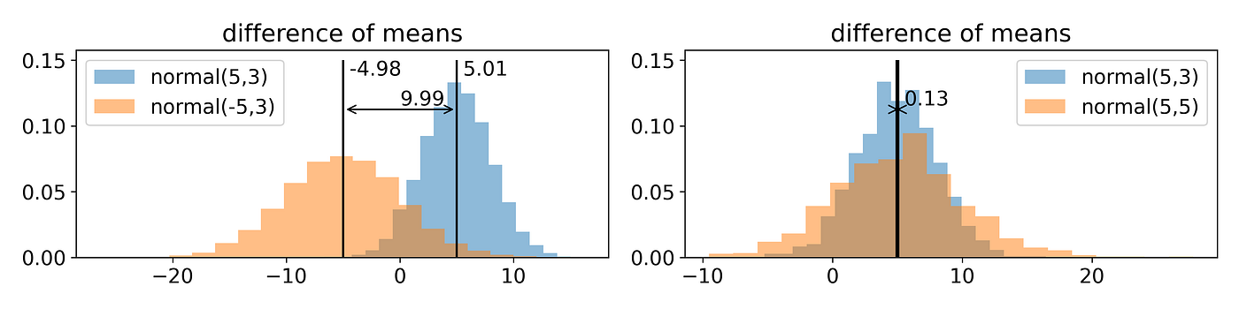
Differences in aggregate statistics like in mean are not metrics in the mathematical sense. A metric would normally require that M(X₁, X₂) = 0 whenever X₁ = X₂ which is a desirable feature for measuring drift as well and one which difference of mean does not respect. A metric that does is Earth-Mover Distance or Wasserstein Distance. The definition is not very insightful but the synonym “earth-mover” is: the metric measures how much earth (probability density) needs to be moved and how far (in units of X₁’s domain) to transform one distribution into the other. An implementation is available in scipy (wasserstein_distance).
Categorical Features
Drift metrics that apply to categorical features (usually) view empirical data as discrete distributions. These are defined in terms of the probabilities associated with each categorical value for a given feature of interest in a distribution. Metrics derived from norms are examples of such metrics:
![\text{NormDistance}_p(X_1, X_2) := \left\| \left< Pr[X_1=x] — Pr[X_2=x] \right>_x \right\|_p](https://miro.medium.com/max/1062/1*Q6LFSNEkIu25Q60M7QfU-w.png)
The base p is usually 1, 2, or infinity. We further discuss these distances in the interpretability section below. Norms are implemented in numerical libraries including numpy (linalg.norm).
The other family of metrics that apply to categorical features are the discrete versions of information theoretic measures which we get into in the next section.
Metrics Origin and Interpretability
Some distance measures are more interpretables than others. The origin of metrics is closely related to the interpretations or intuitions we can apply. We discuss common origins and related interpretations here.
The aforementioned DifferenceOfMeans or difference of any interpretable aggregate statistic have the benefit of being interpretable in terms of their respective aggregate (i.e. mean, deviation, etc.).
Earth-mover distance has an interpretation as noted earlier in the article and can be given interpretable units. If feature X is measured in units u (dollars, miles, etc), Earth-mover distance is measured in u as well (technically it includes a factor of unitless probability) and captures the expected how far (in u) must the distributions be moved to match each other. This has some benefits and some drawbacks. Interpreting an Earth-mover distance of “5000 dollars” may require some understanding of the underlying feature as this might be a small change or a big one depending on what the feature represents. This is also a strength if an analyst does it indeed have some clue about the feature and can connect such a quantity to their experiences (i.e. if the feature is “yearly salary”, a distance of “5000 dollars” should be intuitively interpretable by typical data scientists).
Statistics
The question of “are these distributions the same’’ is often found and answered in the field of statistics. Several of the so-called “tests’’ have thus found their way into ML for measuring drift. Examples include Kolmogorov-Smirnov test and the related statistic, and Chi-squared test. One benefit of statistics-based measures is they come with interpretations in terms of confidence or p-value; indicating not just how much the distributions differ, but a confidence in that observation. Both of these tests are available in scipy (kstest, chisquare).
Information Theory
The other class of metrics comes to us from information theory. Most appropriate is Jensen-Shannon Distance. While the field features numerous measures of distribution difference, their ranges are often infinite or they are not symmetric. JS distance is a symmetric bounded variant of relative entropy (or Kullback-Leibler divergence) with a 0–1 range. Another important aspect of these metrics is that values attained by features are not significant, only their probabilities. For categorical features, for example, Jensen-Shannon distance will not care if you permute your feature values as long as the set of probabilities remains fixed.
Metrics derived from information theory may be associated with units of “bits” or “nits” (depending on which log base was used, 2 or e, respectively) but the relative measures we noted here are not as conveniently interpretable as entropy itself which has connections to encoding length and thus could be said to define the unit “bit”.
Implementations of these measures is available in scipy (entropy, jensenshannon). They are applied to distributions (i.e. lists of probabilities) and thus only operate on categorical features. In the Assumptions or Parameters section we discuss their application to numerical features.
Others sources for Interpretation
Some metrics can be interpreted by, technically unitless, probability. This may not be as intuitive as feature units as in earth mover, it may offer some insight. Several metrics operating on categorical features that interpret empirical distributions as actual probability distributions produce values interpretable as probability. This includes 1-norm and infty-norm distances mentioned above as well as Total Variation Distance (which is identical to half of L₁ norm distance). L₁, for example, tells us the total difference in probability over all categories. L∞, on the other hand, tells us the difference in probability of the most differing category.
p-norm distances have spatial interpretations but they are applied to probability values. If a distribution is a coordinate (with each probability a dimension), then 1-norm distance corresponds to Manhattan distance whereas 2-norm distance is Euclidean distance. While the spatial interpretation may not be very intuitive, the this other property of such norms is more useful:
- In larger bases, p-norm distance emphasizes differences in the most differing dimension / probability. In the extreme ∞-norm, the distance becomes:
![\text{NormDistance}_\infty(X_1, X_2) = \max_x \left| Pr[X_1=x] — Pr[X_2=x] \right|](https://miro.medium.com/max/1060/1*cQdnRMJ3PbSXAZQ5KpcflQ.png)
- In smaller bases, p-norm distance emphasizes the number of dimensions involved in a difference. In the extreme case 0-norm, the distance becomes a count of how many probabilities changed, regardless of by how much. We caution, though, that 0-norm is not useful for measuring drift given its sensitivity to even minuscule changes.
Barring units or probability, some metrics are bounded in a fixed range. All of the metrics mentioned in this article have a minimum of 0 indicating least possible difference (or identical distributions) and save for DifferenceOfMeans and Earth-mover, all of the metrics bounded above with 1, sqrt(2) or some other maximum value indicating the largest possible difference.
Assumptions or Parameters
The use of aggregate statistics as in DifferenceOfMeans above to distinguish distributions comes with assumptions. Specifically, that mean is sufficient to describe the distribution and differences in two distributions. Even normal distributions require an additional variation to fully describe which limits the informativeness of such metrics in general cases. However, simple aggregate differences are still useful given their ease of interpretability (discussed below). Statistical mean may be the first thing we think of when describing a numerical dataset and often enough we need not to consider more.
Another class of assumptions comes from approximations of metrics defined for continuous distributions using discretization. Information-theoretic metrics such as Relative entropy and Jensen-Shannon distance is straightforward to compute for categorical features but is formally defined with an integral for continuous features. A quick fix here is to discretize a continuous value feature into bins and apply a discrete distribution version of a metric to the result. This however now introduces a parameter (the number of bins for example) that can influence the result. While various rules-of-thumb suggest binning strategies (see bins and width), they tend to result in over-estimates of drift.
Metrics break down when the number of bins is set too high. The produced drift results tend to a function of solely of the number of bins and not the actual empirical distributions involved.
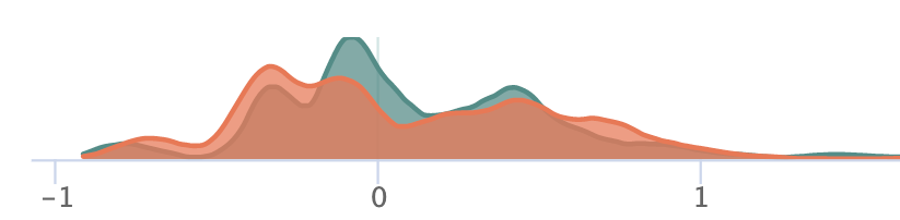
An alternative approach which is not susceptible to binning is via (kernel) density estimation: fit functions to the observed densities and evaluate the distance between these estimated densities instead of binned frequencies. While computing the distance between the estimates also requires binning, this setting becomes less important and in some cases can be set arbitrarily high (for NormDistances at least).
Using density estimation also depends on parameters: what sorts of functions to employ to estimate density? A common approach is a mixture of gaussians parameterized by a bandwidth. An example of such an approach is demonstrated in the below figure with the true densities and estimated densities from samples on the left and the resulting distances on the right. Rules of thumb for setting bandwidth are also available (see The importance of kernel density estimation bandwidth).
Most of the underlying tools necessary to implement the simple binning methods and the kernel density estimated methods are available in numpy and sklearn via histogram and KernelDensity in conjunction with the statistical or information theoretic methods mentioned earlier in this article.
Rare Values
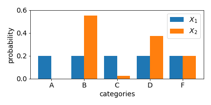
The final aspect of drift metrics we cover in this article is the impact of changes in rare events (rare values). In most metrics, the impact of any change in a categorical value that is rare to begin with is minimal, proportional to its probability in the datasets being compared. As in the example animation below, a categorical feature which during training had value “rareA” in just 10% of the instances, will have generally only 10% impact on a drift measure, even if in the deployment data, the number of instances of this value reduced to 0%. On the other hand, in some metrics, the probability change is considered (multiplicatively) relative to each other and a change from 10% to 0% is significant.

![\text{NormDistance}_p(X_1, X_2) := \left( \Sigma_x \left| \overbrace{\Pr[X_1=x] — \Pr[X_2=x]}^{\text{A: additive difference}} \right|^p \right)^\frac{1}{p}](https://miro.medium.com/max/1140/1*OBr-zyKeWchZYNG4roY6dQ.png)
Looking under the hood of example metric definitions, RelativeEntropy and NormDistance, we see two elements: an expectation over train split values (part A) or an additive difference between train/test probabilities (as in NormDistance) and in some cases a relative component that compares the probability of a value in train vs in test (part B). The first term is responsible for limiting the impact of rare values while the latter can highlight differences in rare values if their relative probabilities change significantly. Most categorical metrics feature part A, but not all feature the relative component of part B.
Metrics that feature B include Relative Entropy, Jensen Shannon Divergence, and Population Stability Index. For some metrics, the drift measured in case of an event going from >0% to 0% representation between datasets can be technically unbounded (due to division by 0 in definitions). One can avoid these by incorporating small additive constants to all probabilities or at least ones in the denominator positions.
Summarizing
- A variety of drift metrics can help you detect and quantify data drift, having varied application, interpretations, origins, and other aspects that may be salient to your application.
- The interpretation of metrics varies and some knowledge of the field from which they derive may be helpful towards understanding those metrics.
- Metrics are often approximations, especially metrics for numerical or continuous features, and may make some assumptions to be conveniently computable and may require setting parameters.
- While some metrics do not capture relatively large drift in rare categories, others drift metrics are able to highlight such changes.
For your reference, here is a list summarizing the drift metrics mentioned in this article and the salient features we have discussed:
NormDistance
- Origin: Geometry
- Feature Types: Categorical, *Numerical with assumptions
- Interpretation: distance; p=0 (not recommended); p=1 (Manhattan Distance); p=2 (Euclidean Distance); p=∞ (maximal probability shifted)
- Relative: No
- Tools: numpy linalg.norm
Relative Entropy / Kullback-Liebler Divergence
- Origin: Information Theory
- Feature Types: Categorical, *Numerical with assumptions
- Interpretation: bits/nits, permutation invariant
- Relative: Yes
- Tools: scipy entropy
Jensen-Shannon Distance
- Origin: Information Theory
- Feature Types: Categorical, *Numerical with assumptions
- Interpretation: bits/nits, permutation invariant
- Relative: Yes* (technically yes but effectively no: JS Distance uses Relative Entropy between one input distribution and the mid-point between the two input distributions; the result is that even a disappearing value will have limited impact as the relative term for it is bounded by 1)
- Tools: scipy jensenshannon
Total Variation Distance
- Origin: Probability Theory
- Feature Types: Categorical, *Numerical with assumptions
- Interpretation: Same as NormDistance with base 1
- Relative: No
- Tools: numpy linalg.norm
DifferenceOfMeans
- Origin: Statistics
- Feature Types: Numerical
- Interpretation: same units as feature value
- Relative: No
- Tools: numpy mean
Earth-Mover Distance / Wasserstein Distance
- Feature Types: Numerical
- Interpretation: same units as feature value
- Relative: No
- Tools: scipy wasserstein_distance
Kolmogorov-Smirnov Test
- Origin: Statistics
- Feature Types: Numerical
- Interpretation: statistical confidence available
- Relative: No
- Tools: scipy kstest
Chi-square Test
- Origin: Statistics
- Feature Types: Numerical
- Interpretation: statistical confidence available
- Relative: No
- Tools: scipy chisquare
* Categorical Metrics for Numerical Features
- Tools: numpy histogram, sklearn KernelDensity
This blog has been republished by AIIA. To view the original article, please click HERE.
Recent Comments