
Overview
Generating business value is key for data scientists, but doing so often requires crossing a treacherous chasm with 90% of models never reaching production (and likely even fewer providing real value to the business). The problem of overfitting is a critical challenge to surpass, not only to assist ML models to production status but also to create a generalizable model that provides lift in the real world. A model exhibits overfitting if it memorizes patterns in training instances that do not generalize to new data, and machine learning models are more prone to overfitting because they have greater capacity to learn complex relationships.
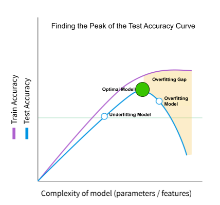
Some improvements such as fixing mislabeled data or adding more data can shift the accuracy curve up while others allow us to move along the accuracy curve, as shown above. As we move along the accuracy curve, we explicitly toggle between reducing bias (to the left) and reducing variance (to the right) in the hope of finding the most performant general model (the green dot). We should also be cognizant that fitting a large number of models with the same test set can also degrade the generalizability of our model.
A large gap between train and test accuracy does not necessarily indicate poor performance, and the optimal model (at the peak of the test accuracy curve) may even have a large train-test gap. Inspecting the reasons for the performance gap can not only be used to reduce general overfitting, but it can also be informative for correcting overfitting for edge cases in the training data. This article will demonstrate how we can identify areas for improvement by inspecting an overfit model and ensure that it captures sound, generalizable relationships between the training data and the target. The goal for diagnosing both general and edge-case overfitting is to optimize the general performance of our model, not to minimize the train-test gap.
Introduction to the Airbnb Price Prediction Series
This is the first installment of a new series utilizing Airbnb data scraped by Inside Airbnb and hosted by OpenDataSoft. Pricing a rental property is a challenging task for Airbnb owners as they need to understand the market, the features of their property, and how those features contribute to listing price. The models we develop and improve in this series will focus on improving a pricing model for Airbnb listings.
I will build a simple benchmark model that overfits on the training data split, and then utilize TruEra to find the root cause of overfitting, and assess improvement on that axis. Along the way, I’ll also demonstrate using the requests get method to access the data from OpenDataSoft, the use of sklearn pipelines for preprocessing and modeling steps, and how to tune hyperparameters using the hyperopt package.
Retrieve the Data
After importing the required packages, we’ll want to pull in our data. To do this, we will use the requests package, supplying the target url to get the data from. After receiving the json response, we’ll flatten the response and reformat it as a pandas dataframe.
| import requests | |
| import pandas as pd | |
| def get_airbnb_data(city): | |
| #input city with + instead of spaces, e.g. “San+Francisco” | |
| #note: open data soft caps requests at 10,000 | |
| url = “https://public.opendatasoft.com/api/records/1.0/search/?dataset=airbnb-listings&q=&rows=10000&refine.city=” + city | |
| resp = requests.get(url) | |
| print(resp.status_code) | |
| data = resp.json() | |
| abnb_df = pd.DataFrame([flatten_json(x,exclude=‘datasetid’) for x in data[‘records’]]) | |
| return abnb_df |
Pre-Processing
Next we want to drop a small subset of unlabeled data and columns that are missing greater than 75% of their values.
| #drop unlabeled data | |
| abnb_pre = abnb_df.dropna(subset=‘price’) | |
| # Delete columns containing either 75% or more than 75% NaN Values | |
| perc = 75.0 | |
| min_count = int(((100–perc)/100)*abnb_pre.shape[0] + 1) | |
| abnb_pre = abnb_pre.dropna(axis=1, thresh=min_count) |
It’s pre-processing time! Let’s set up our transformers. For this data, we’ll need transformers to drop features, set up one-hot transformers, convert dates to days, and fill NANs with zero where applicable.
After building out transformers, the next step is to instantiate and then build sklearn pipelines with the instantiated transformers as steps. When building pipelines, it can be more readable to “stack” our pipelines rather than creating a single longer pipe.
| from sklearn.pipeline import Pipeline | |
| #instantiate transformer classes | |
| cat_onehot_transformer = cat_onehot_transformer_custom(cat_list) | |
| url_onehot_transformer = url_onehot_transformer_custom(url_list) | |
| convert_dates_transformer = convert_dates_transformer_custom(date_list) | |
| to_float_transformer = to_float_transformer_custom(tofloat_list) | |
| fillna_transformer = fillna_transformer_custom(fillna_list) | |
| cap_reviews_per_month = cap_reviews_per_month_custom() | |
| drop_features = drop_features_selector(drop_list) | |
| #set up pipelines | |
| cat_preprocessing_pipe = Pipeline(steps = [ | |
| (‘cat_onehot_transformer’, cat_onehot_transformer), | |
| (‘url_onehot_transformer’, url_onehot_transformer) | |
| ]) | |
| num_preprocessing_pipe = Pipeline(steps = [ | |
| (‘convert_dates_transformer’,convert_dates_transformer), | |
| (‘to_float_transformer’,to_float_transformer), | |
| (‘fillna_transformer’,fillna_transformer), | |
| (‘cap_reviews_per_month’, cap_reviews_per_month) | |
| ]) | |
| # combine both numerical and categorical preprocessing step | |
| combined_preprocessing = Pipeline([ | |
| (‘drop_features’, drop_features), | |
| (‘numericals’, num_preprocessing_pipe), | |
| (‘categoricals’, cat_preprocessing_pipe) | |
| ]) |
Last, we need to make sure any new data where we use the model for predictions contains the same columns as the training data, while preventing one hot encodings from our test step from leaking to our training data. To do that, we’ll build one last transformer that re-indexes the data on only the training columns, and add it to our preprocessing pipeline.
| class comprehensive_features_custom(BaseEstimator, TransformerMixin): | |
| def __init__(self, comprehensive_features): | |
| self.comprehensive_features = comprehensive_features | |
| def fit(self, X, y = None): | |
| return self | |
| def transform(self, X): | |
| X_post = X.reindex(labels=comprehensive_features, axis=1) | |
| return X_post | |
| set_comprehensive_features = comprehensive_features_custom(comprehensive_features) | |
| #comprehensive preprocessing pipe | |
| comprehensive_preprocessing = Pipeline([ | |
| (‘combined_preprocessing’,combined_preprocessing), | |
| (‘set_comprehensive_features’,set_comprehensive_features) | |
| ]) |
TruEra Set Up
After we’ve set up our preprocessing pipelines, next we want to set up our project in Truera, and add our train and test data splits to a data collection.
| import truera | |
| #set up TruEra workspace | |
| from truera.client.truera_workspace import TrueraWorkspace | |
| from truera.client.truera_authentication import BasicAuthentication | |
| auth = BasicAuthentication(USERNAME, PASSWORD) | |
| tru = TrueraWorkspace(CONNECTION_STRING, auth, verify_cert = False) | |
| tru.set_environment(“remote”) | |
| tru.set_project(“airbnb_sf_price”, score_type=“regression”) | |
| #create data collection or schema | |
| tru.add_data_collection(data_collection_name = “sf_data_collection_v1”, | |
| pre_to_post_feature_map = feature_map_data, | |
| provide_transform_with_model=True) | |
| #add data splits to collection | |
| tru.add_data_split(“train”, pre_data = X_train, label_data=y_train, split_type=“train”) | |
| tru.add_data_split(“test”, pre_data = X_test, label_data=y_test, split_type=“test”) |
XGBoost Model Pipeline
Last, all we need to do is instantiate an xgboost model as our benchmark and add it to our pipeline. Then we’ll fit the pipeline and add it to TruEra.
| #instantiate model | |
| xgb_reg = xgb.XGBRegressor() | |
| # combine both preprocessing and modeling | |
| xgb_pipe = Pipeline([ | |
| (‘preprocess’, comprehensive_preprocessing), | |
| (‘xgboost’, xgb_reg) | |
| ]) | |
| #fit pipe | |
| xgb_pipe.fit(X_train,y_train) | |
| #add model to truera | |
| tru.add_python_model(“xgb_pipe”, xgb_pipe, pipeline_feature_map = feature_map_data) |
Now we’re ready to evaluate our model using TruEra!
Diagnosing an Overfitting Model
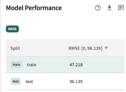
With complex ML models able to memorize large parts of the training set, the training accuracy is an insufficient indicator of model performance. Overfitting can occur in these cases, where model performance on the training dataset is improved at the cost of performance on unseen data. Overfitting is critical for data scientists to diagnose before models reach production, as degraded performance then becomes much more costly. After quickly taking a look at the performance on both the train and test data splits, we observe a large gap in performance – the root mean squared error for our train set is 58.766 with 97.402 for test, a sixty-five percent gap. While this gap isn’t necessarily due to overfitting, this gives us a hint that we should investigate its root cause.
Bucketization of Numerical Features
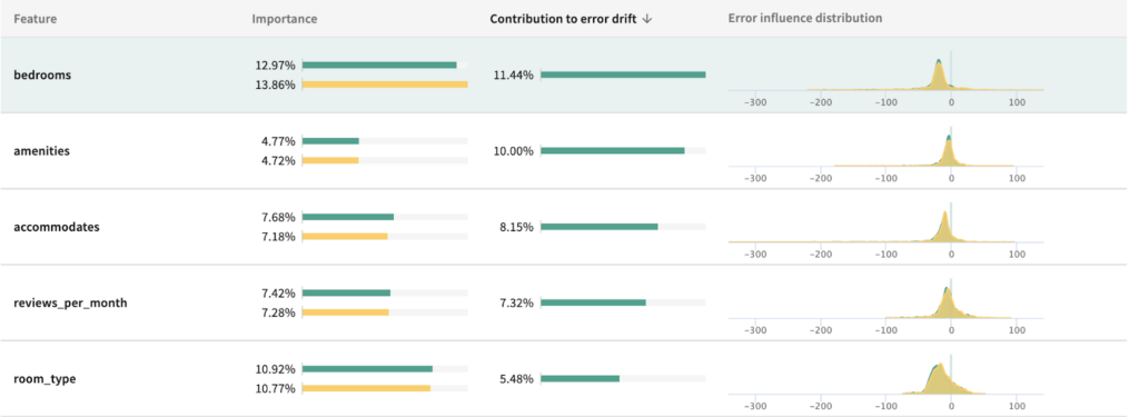
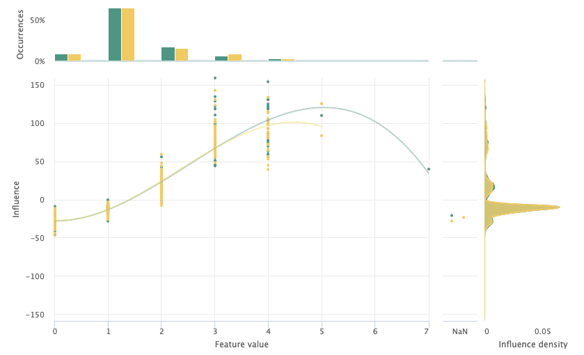
Using TruEra Diagnostics, the largest contributor to error drift is bedrooms, contributing 11.44% to the error drift of the test set compared to train.
Looking at the influence sensitivity plot, we observe thin data in the 3+ bedrooms range. To counteract this issue, we’ll convert this feature to categorical where 3+ bedrooms are bucketed as one category. The features “accomodates” and “bathrooms” also fall into this pitfall, and we’ll bucket accordingly.
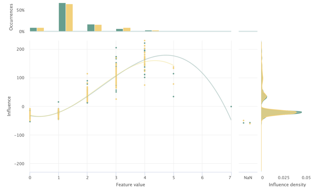
To bucketize these features, I’ll create a new transformer class called bucketize_features_custom, and then use pandas cut to bin each value range to its respective label. After making this change, we can see in the resulting ISP that the positive influence of points on the higher end of the feature distribution. We can also observe a noticeably more similar influence density between the train and test split in the ISP resulting from this change, shown below.
Restructure Categorical Encodings to Reduce Overparameterization
Referring back to the largest contributors to error drift, second on the list is amenities. Clicking into that feature, we observe that the feature is overparameterized in that every unique combination of options is being treated as a separate category. To fix this issue, we need to adjust our encoder to account for comma-separated multi-hot encodings.
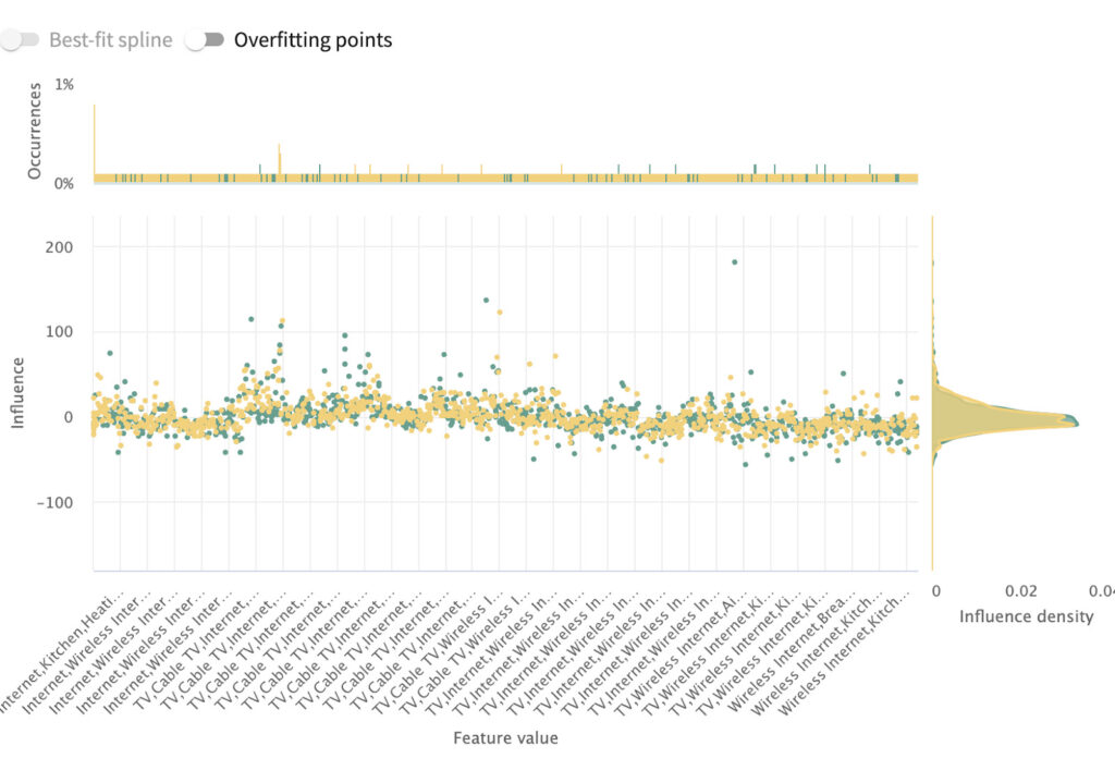
We’ll assume that the normal categoricals do not contain commas in their values so that we can build a single transformer that handles both cases. Updating the transformer here will resolve similar issues for other features as well, including “Features”, and “Host Verifications”.
| from sklearn.base import BaseEstimator, TransformerMixin | |
| class cat_onehot_transformer_custom(BaseEstimator, TransformerMixin): | |
| def __init__(self, cat_list): | |
| self.cat_list = cat_list | |
| def fit(self, X, y = None): | |
| return self | |
| def transform(self, X): | |
| X_post = X.copy() | |
| for cat in self.cat_list: | |
| X_post[cat] = X_post[cat].str.replace(‘ ‘, ‘_’) | |
| #sometimes check-all-that-apply style, separated by ‘,’ | |
| cat_onehot = X_post[cat].str.get_dummies(sep=‘,’).rename(lambda x: cat + ‘_’ + x, axis=‘columns’) | |
| X_post[cat] = np.nan | |
| X_post = X_post.join(cat_onehot) | |
| return X_post |
Remove Non-Influential Features
After adjusting for the encodings, we noticed that there are a large number of features with close to zero influence on the model. Somewhat arbitrarily, I choose to remove features with less than 1% influence. Below you can see that the train RMSE has improved significantly by approximately 11 points, while the test performance improved slightly by one point.
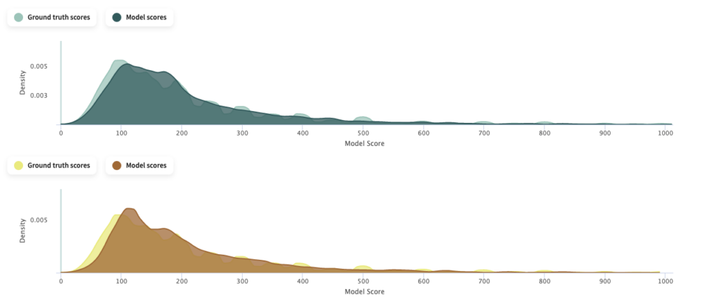
Let’s also take a look at how our predictions relative to ground truth moved. The updated model is shown in green compared to the baseline in yellow. With this comparison, we can observe that the updated model shows a flatter distribution of predicted listing prices around $100, as well as an increase in density of predicted lower listing prices which more closely mirrors ground truth.
HyperParameter Tuning
As you can see above, so far we’ve been unable to resolve the dropoff in performance between train and test. Next, we’ll turn to hyperparameter tuning to look for a set of hyperparameters with improved test performance. To do so, we’ll tune outside of the sklearn pipeline and utilize the hyperopt package. First, we’ll set the space for the hyperparameters we’re looking to tune. For this model, I will tune max_depth, gamma, reg_alpha, reg_lambda, and min_child_weight. You can find more information on the parameters in the xgboost documentation.
| from hyperopt import STATUS_OK, Trials, fmin, hp, tpe | |
| #use post data instead of pipe for hyperparameter tuning, get x_test_post | |
| X_test_post = comprehensive_preprocessing.fit_transform(X_test, y_test) | |
| #set hyperparameter space | |
| space={‘max_depth’: hp.quniform(“max_depth”, 3, 18, 1), | |
| ‘gamma’: hp.uniform (‘gamma’, 0, 18), | |
| ‘reg_alpha’ : hp.uniform(‘reg_alpha’, 0,1), | |
| ‘reg_lambda’ : hp.uniform(‘reg_lambda’, 0,2), | |
| ‘min_child_weight’ : hp.uniform(‘min_child_weight’, 0, 20), | |
| ‘n_estimators’: 1000, | |
| ‘seed’: 0 | |
| } |
After setting the hyperparameter space, next we need to define the objective, and define root mean squared error as our loss metric. Then, all we need to find the minimum of that objective in the hyperparameter space.
| #define the objective function and the hyperparameters we want to tune | |
| def objective(space): | |
| model=xgb.XGBRegressor( | |
| n_estimators =space[‘n_estimators’], | |
| max_depth = int(space[‘max_depth’]), | |
| gamma = space[‘gamma’], | |
| reg_alpha = int(space[‘reg_alpha’]), | |
| min_child_weight=int(space[‘min_child_weight’]) | |
| ) | |
| evaluation = [( X_train_post, y_train), ( X_test_post, y_test)] | |
| model.fit(X_train_post, y_train, | |
| eval_set=evaluation, eval_metric=“mae”, | |
| early_stopping_rounds=10,verbose=False) | |
| pred = model.predict(X_test_post) | |
| rmse= math.sqrt(mean_squared_error(y_test, pred)) | |
| print (“SCORE:”, rmse) | |
| return {‘loss’:rmse, ‘status’: STATUS_OK, ‘model’: model} | |
| trials = Trials() | |
| best_hyperparams = fmin(fn = objective, | |
| space = space, | |
| algo = tpe.suggest, | |
| max_evals = 100, | |
| trials = trials) | |
| print(“The best hyperparameters are : “,“\n“) | |
| print(best_hyperparams) |
Last, we’ll just specify the best hyperparameters in our xgboost regression, insert it back into the sklearn pipeline, and upload to TruEra.
| #instantiate model | |
| xgb_reg = xgb.XGBRegressor( | |
| gamma = 9.525156702124235, | |
| max_depth = 3, | |
| min_child_weight = 9.517754381682627, | |
| reg_alpha = 0.07435977523021892, | |
| reg_lambda = 1.4770738953975366) | |
| # combine both preprocessing and modeling | |
| xgb_pipe = Pipeline([ | |
| (‘preprocess’, comprehensive_preprocessing), | |
| (‘xgboost’, xgb_reg) | |
| ]) | |
| xgb_pipe.fit(X_train, y_train) | |
| #add model to truera | |
| tru.add_python_model(“xgb_pipe_tuned_v3”, xgb_pipe, pipeline_feature_map = feature_map_data) |
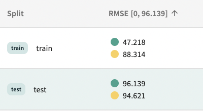
Evaluate the Performance of the Tuned Model
Now that we’ve tuned the hyperparameters of our xgboost regression, we’ve again improved the performance on the test set. While this was at the cost of drastically reducing the performance on the training dataset, we’re okay with this tradeoff. The objective is not to maximize the performance of the model on seen data, but to improve performance on unseen data and ultimately in production. While there still exists a gap in performance between the train and test split, we have made model improvements to correct edge-case and general overfitting. Exact requirements for promoting a given model to production are context-specific and out of scope for this article but we can now proceed with confidence that the complex relationships captured by our ML model are generalizable.
Next Time…
Later in the series, we’ll build a framework for standardized model testing, assess transfer learning and more. Stay tuned!
Learn More!
If you’re interested in learning more about how to explain, debug and improve your ML models, apply to get early access to TruEra diagnostics or join the community!
This blog has been republished by AIIA. To view the original article, please click here: https://truera.com/practical-guide-for-debugging-overfitting-in-ml/
Recent Comments