Synthetic Time-Series Data: A GAN approach

Generate synthetic sequential data with TimeGAN

Time-series or sequential data can be defined as any data that has time dependency. Cool, huh, but where can I find sequential data? Well, a bit everywhere, from credit card transactions, my everyday routine and whereabouts to medical records, such as ECG and EEG’s. Although sequential data is pretty common to be found and highly useful, there are many reasons that lead to not leverage it — from privacy regulations to the scarcity of its existence.

In one of my previous posts, I’ve covered the ability of Generative Adversarial Netoworks (GANs) to learn and generate new synthetic data that preserves the utility and fidelity of a real datasets, nevertheless to generate tabular data is far more simple than generating datasets that should preserve temporal dynamics. To model successfully time-series data means that a model must, not only capture the datasets features distributions within each time-point but also, it should be able to capture the complex dynamics of those features across time. We must not forget also that each time sequence as a variable length associated.

But being a challenging task, does not mean it is impossible! Jinsung Yoon and Daniel Jarret have proposed, in 2019, a novel GAN architecture to model sequential data — TimeGAN — that I’ll be covering with a practical example throughout this blog post.

Time-series Generative Adversarial Networks

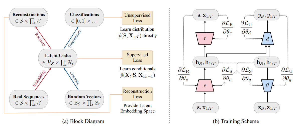
TGAN or Time-series Generative Adversarial Networks, was proposed in 2019, as a GAN based framework that is able to generate realistic time-series data in a variety of different domains, meaning, sequential data with different observed behaviors. Different from other GAN architectures (eg. WGAN) where we have implemented an unsupervised adversarial loss on both real and synthetic data, TimeGAN architecture introduces the concept of supervised loss —the model is encouraged to capture time conditional distribution within the data by using the original data as a supervision. Also, we can observe the introduction of an embedding network that is responsible to reduce the adversarial learning space dimensionality.

What’s new about TimeGAN?

Different from other GAN architectures for sequential data, the proposed framework is able to generate it’s training to handle a mixed-data setting, where both static (attributes) and sequential data (features) are able to be generated at the same time.

Less sensitive to hyper parameters changes

A more stable training process, when compared to other architectures.

Implementation with TensorFlow 2

As mentioned above, TimeGAN is a framework to synthesize sequential data compose by 4 networks, that play distinct roles in the process of modelling the data: the expected generator and discriminator, but also, by a recovery and embedder models.

For the purpose of this example, I’ve decided to keep it simple with a very similar architecture for all the 4 elements: A 3 layers GRU network. But it’s possible to have this architectures change to more or less layers, and also to chose between GRU and LSTMs.

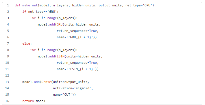
Which results in the definition of each of the networks elements as per the code snippet below.

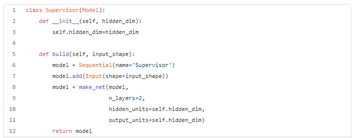
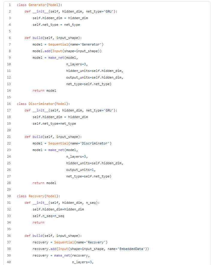
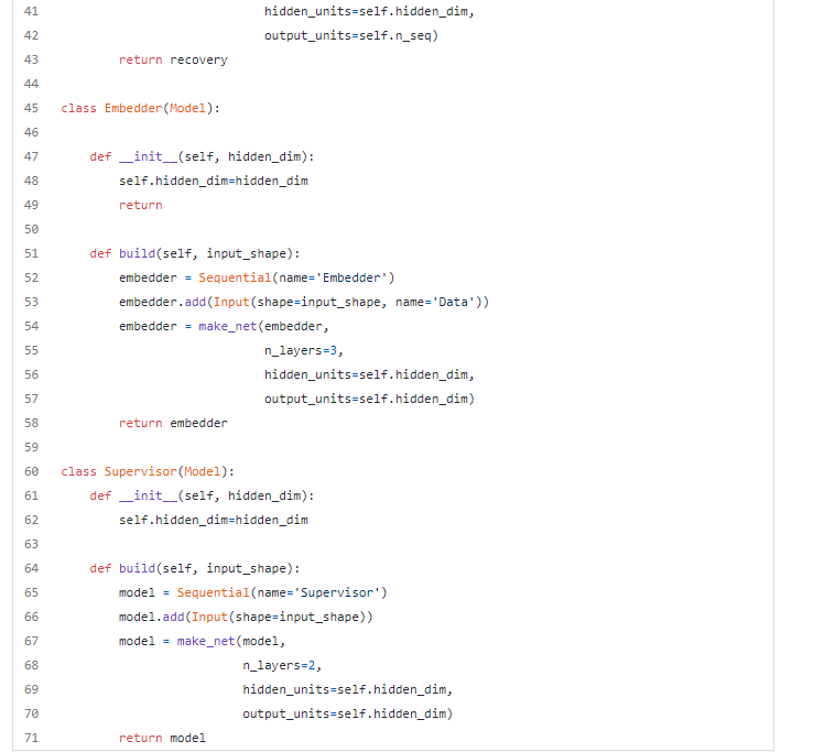
In what concerns the losses, the TimeGAN is composed by three:

• The reconstruction loss, which refers to the auto-encoder (embedder & recovery), that in a nutshell compares how well was the reconstruction of the encoded data when compared to the original one.
• The supervised loss that, in a nutshell, is responsible to capture how well the generator approximates the next time step in the latent space.
• The unsupervised loss, this one it’s already familiar to us, a it reflects the relation between the generator and discriminator networks (min-max game)

Given the architecture choice and the defined losses we have three training phases:

1. Training the autoencoder on the provided sequential data for optimal reconstruction
2. Training the supervisor using the real sequence data to capture the temporal behavior of the historical information, and finally,
3. The combined training of four components while minimizing all the three loss functions mentioned previously.

The full code detailing the training phases can be found at ydata-synthetic.

The original implementation of TimeGAN can be found here using TensorFlow 1.

Synthetic stock data

The data used to evaluate the synthetic data generated by the TimeGAN framework, refers to Google stock data. The data has 6 time dependent variables: Open, High, Low, Close, Adj Close and Volume.

Prior to synthesize the data we must, first, ensure some preprocessing:

1. Scale the series to a range between [0,1]. For convenience, I’ve decided to leverage scikit-learn’s MinMaxScaler;
2. Create rolling windows — following the original paper recommendations, I’ve create rolling windows with overlapping sequences of 24 data points.

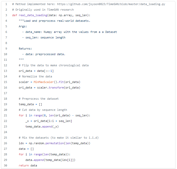
Following the recommendations from the original paper, I’ve decided to train the synthesizer for 10000 iterations nevertheless, bare in mind, that these values must the optimized for each data set in order to return optimal results.

You can find in this notebook the full flow including the data download, processing and synthesizing.

Measuring synthetic data fidelity and utility

Now that we were able to synthesize our data, it’s time to check whether the new data is able to reproduce properly the behavior observed in the original stock data data.

Visual comparison

One of my favorites ways to compare real with synthetic data is through visualization. Of course that in terms of automation is not the ideal to validate the quality of the new synthetic data, but it gives us already a pretty good idea. To ensure a 2D visualization of the results, it was applied both a TSNE and a PCA with 2 components.

The results are pretty promising, as we see an almost perfect overlap between the synthetic and the real data points.

Synthetic data utility — Train synthetic test real

There are a plenty of different metrics that can be used to measure the utility of the data such as the SRA and the TSTR.

In this example we’ve decided to go for the TSTR method to validate the utility of our synthetic data. To be used as a regressor model, I’ve decided for a simple architecture with a single layer GRU with 12 units.

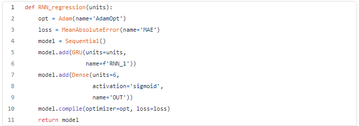
Prior to train the model, we had to prepare the inputs:

• 75% of the data was used as train data (for both synthetic and real datasets)
• 25% of the real data was used as the test set.

For both the model trained on synthetic and the one trained on the real data, I’ve used as the validation set loss as the early stopping criteria. Below are the summarized results obtained for the test set.

Conclusion

The results obtained with this experiment are very promising and exciting in what concerns the generation of synthetic sequential data. Nevertheless, there are a few caveats that are needed to be pointed: the data under study can be considered to be quite simple, as it was relatively small, with a daily time frequency, there were no surprises in terms of missing values and the dimensionality (columns wise) was relatively low. Not to mention, the very intensive training time.

But without a doubt, Generative Adversarial Networks are impressive frameworks, that can be leveraged for much more than synthetic data generation. For those of you, that are looking to keep exploring synthetic data generation have a look into our GitHub repository. We’ll be updating it with new generative algorithms as well as new data, and we invite you to collaborate!

This blog has been republished by AIIA. To view the original article, please click HERE.