In our last post we took a broad look at model observability and the role it serves in the machine learning workflow. In particular, we discussed the promise of model observability & model monitoring tools in detecting, diagnosing, and explaining regressions models that have been deployed to production.
This leads us to a natural question of: what should I monitor in production? The answer, of course, depends on what can go wrong.
In this article we will be providing some more concrete examples of potential failure modes along with the most common symptoms that they exhibit in your production model’s performance.
As with most things in the world, a model’s task is likely to change over time. Concept Drift or Model Drift is a model failure mode that is caused by shifts in the underlying task that a model performs, which can gradually or suddenly cause a regression in the model’s performance.
Concept Drift Example
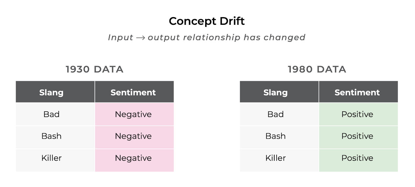
To put it a bit differently, the task that your model was trained to solve may not accurately reflect the task it is now faced in production.
For example, imagine that you are trying to predict the sentiment of a particular movie review and your model was trained on reviews from the early 1970s. If your model is any good, it has probably learned that the review, “Wow that movie was bad”, carries negative sentiment; however fast forward into the world of 1980s slang, and that exact same review might mean that the movie was fantastic.
So the input to the model didn’t change, but the result did — what happened? The fundamental task of mapping natural language to sentiment has shifted since the model was trained, causing the model to start making mistakes where it used to predict correctly.
This shift can happen gradually over time, but as we are too often reminded these days, the world doesn’t always change gradually. This fundamental unpredictability about when exactly concept drift is going to happen necessitates a good suite of model monitoring tools.
If you notice that not much has changed in the distribution of your model inputs, yet your model performance is regressing, concept drift may be a contributing factor.
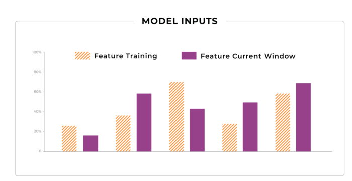
Data lies at the very center of model creation, and data practices can make or break how a model performs in production. In the real world, the distribution of your model’s inputs are almost certain to change over time, which leads us to our next model failure mode: Data Drift or Feature Drift.
Feature Drifting from Training
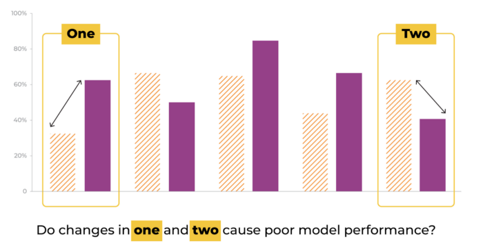
Let’s imagine you’ve just deployed a model that predicts how many streams an album is going to get in its first day on Spotify or Apple Music. Now that your model has been deployed to production for a while, and has been correctly predicting Drake’s meteoric smash hits, you start to notice that your model is starting to make some dramatic mistakes.
Feature Drift Causing Model Performance Issues
After some inspection you notice that some new artists and trendy genres are attracting a majority of the streams, and your model is making large mistakes on these albums.
So what could have possibly gone wrong?
The distribution in your model’s inputs are statistically different from the distribution on which it was trained. In other words, your data has drifted and your model is now out of date. Just like concept drift, data drift can creep up on your model slowly or hit it hard and fast.
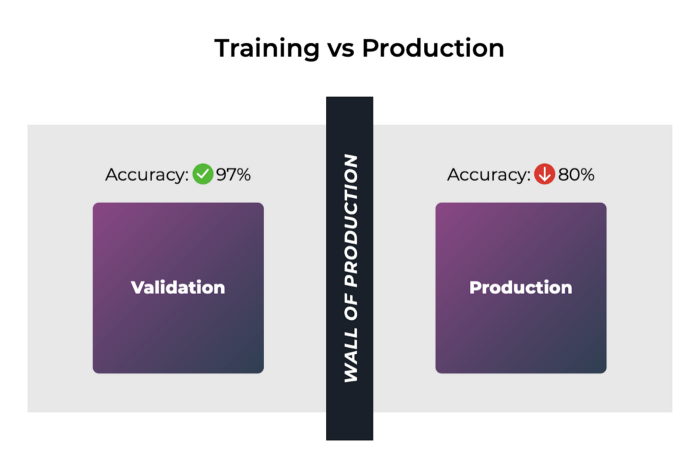
One important thing to mention is that it’s quite common to confuse data drift with training-prod skew. Training-prod skew is when the distribution of your training data differs meaningfully from the distribution of production data. Going back to our previous example, if you had only trained your album model with country music, it will likely not perform well when it sees a new jazz album hit the discovery tab.
Training-production Skew
In both the case of data drift and training-prod skew, the model is experiencing a distribution of model inputs in production that it did not see while training, which can lead to worse performance than when validating the model. So how can we tell the difference?
If your model is unable to achieve close to its validation performance as soon as you deploy you model, you likely are facing training-prod skew, and you might want to rethink your data sampling techniques to curate a more representative dataset; however if your model match has exhibited good production results in the past and you are seeing a slow or sudden dip in performance, it’s very possible that you are dealing with the effects of data drift.
Cascading Model Failures
As machine learned models take the world by storm, it has become more and more common for products to contain a number of machine learned components. In many cases the output of one model is even used directly or indirectly as an input to another model.
Since these models are often trained and validated separately on their own datasets, a head-scratching failure mode is bound to pop up. While both models’ performance can improve in their offline validation performance, they can regress the product as a whole when deployed together.
To demonstrate this concept, let’s pretend that you work on Alexa. Your team is responsible for a speech recognition model that transcribes a user’s speech into text, while a partner team is responsible for classifying these transcribed queries into an action that Alexa can perform for the user.
One day, you discover a breakthrough that improves your team’s speech recognition results by 10% on the validation datasets; however, when you get back to your desk the next day after deploying the updated model you see a huge regression in Alexa’s accuracy in selecting the action that the user requested.
What happened? Well, in making this change to the speech recognition model, the output distribution of the transcribed utterances changed in a statistically significant way. Since these outputs are the inputs to the action classification model, this caused the action predictions to regress, causing your users to sit through a terrible song when they just wanted to set a timer.
To diagnose these cascading model failures, a model observability tool must be able to track the changes to the input and output distributions of each model to be able pinpoint which model introduced the regression in overall performance.
In the previous sections we have been primarily concerned with group statistics surrounding the model’s performance; however, sometimes how your model is performing on a few examples is more concerning.
In an ideal world, there would be no surprises when you deploy your model to production. Unfortunately, we do not live in an ideal world. Your model will likely face anomalous inputs and occasionally produce anomalous results.
Sometimes finding these examples are like finding a needle in a haystack. You can’t address the underlying problem in your model if you can’t find it.
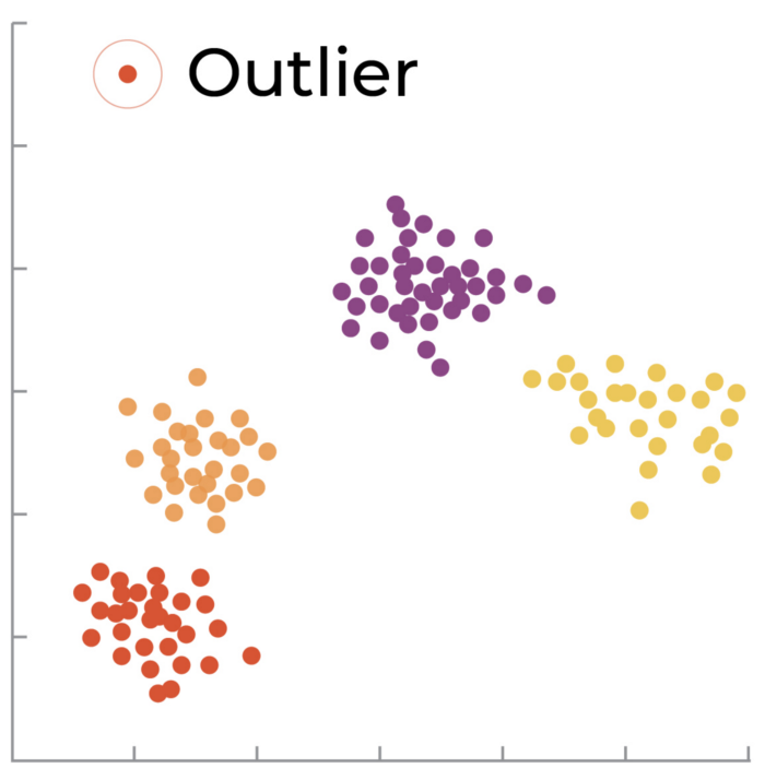
Outlier: Lower Dimensional Mapping
Understanding outliers is typically viewed as a multivariate analysis across all of the input features finding individual predictions that are outliers. Contrast this with the drift description above which is really a general statistic of a single feature over a group of predictions.
Drift: Group of Predictions — Univariate statistic on a feature or model output
Outlier: Individual Prediction or Small Group of Predictions — Multivariate analysis across features
Model owners need a line of defense to detect and protect against these nasty inputs. One technique to accomplish this is to employ an unsupervised learning method to categorize model inputs and predictions, allowing you to discover cohorts of anomalous examples and predictions.
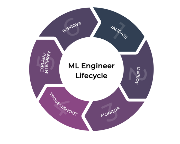
This is where model observability tools shine in helping you tighten your training, evaluating, deploying, and monitoring loop.
If you are seeing a number of examples that don’t fit well into the groups of the more prototypical examples, this could be evidence of some edge cases your model has never seen. In either case these examples may be good candidates for you to include and potentially upsample in your training to shore up these gaps.
Anomalous examples can occur just by chance, but they can also be generated by an adversary who is trying to trick your model. In many business critical applications, especially in the financial sector, model owners have to be hyper-vigilant to monitor for adversarial inputs that are designed to make a model behave in a certain way.
In 2018, Google brought attention to adversarial attacks on machine learned image classification models by demonstrating how a small amount of noise, imperceptible to the human eye, added to an image could cause the model to wildly misclassify.
In applications where every hour counts, the speed in which you can identify a new attack, patch the vulnerability, and redeploy your model may make all the difference in the success of your business.
In summary, there are a number of model failure modes to be on the lookout for, and they rarely affect your model in isolation. To piece together why your model’s performance may have degraded or why your model is behaving erratically in particular cases, you must have the proper measurements to piece together what’s going on. Model monitoring tools fill this role in the machine learning workflow and empower teams to constantly improve your models after they’ve been shipping into the world.
This blog has been republished by AIIA. To view the original article, please click HERE.
Originally published at https://towardsdatascience.com on February 22, 2021.

Recent Comments